Challenges of hard real-time software testing

Hard real-time embedded software presents particular challenges for testing. When the software also implements complex algorithms, testing that these algorithms are correctly implemented across the complete range of possible inputs and operating states can be difficult. Additionally it is often the case that this type of software executes in a loop, with the output of each execution depending not only on the current inputs, but also on the outputs from previous executions.

Verifying that complex current control algorithms are correctly implemented solely by running on the final target hardware is not an effective approach. It is difficult to exercise the software across its full operational envelope on a hardware test system. It is therefore necessary to also unit/module test the software to demonstrate that the specified algorithms are correctly implemented.

To unit or module test software requires knowledge of the expected outputs for each test case. For complex real-time software in which the output depends on previous outputs, calculating the expected outputs for all test cases can be a very laborious task. Once we have decided on a set of tests and test cases (sets of input values), we need to have a way to work out exactly what are the expected outputs in response to each test case.  We want to test behaviour across multiple executions of the loop, so we need to know what the expected outputs across time are, for a set of inputs that may also be changing across time.   I suggest that the best way to do this is to use an executable mathematical model.

There are several suitable modeling tools available, such as MatLab/Simulink, MapleSim and Altair Embed.  There are also open-source options such as Xcos and Scicos that are quite adequate for this purpose.

Introduction to Xcos – x-engineer.org

Scicos Homepage

Once we have an executable mathematical model of the control loop we want to test, we can either execute the model to generate sets of inputs and expected outputs for our module test cases.  Or, if with some additional work we could execute the model at the same time as the control loop to carry out back-to-back testing.

An example of a hard-real time embedded application involving complex algorithms is Field Oriented Control of an electric motor. Model-based testing of this example is discussed here.

Model Based Testing of a Motor Current Control Loop

Motivation

Motor control applications always require high reliability and are frequently safety related. Thorough testing is therefore essential. However, testing of motor control software, particularly at the current control level where execution cycles are fast and timing is critical, presents challenges.

A common type of motor control for brushless AC motors is Field Oriented Control (also known as vector control). In this control method, software is used to tightly control the magnetic fields in the motor via pulse width modulated outputs to bridge hardware that drives current through the motor windings. This allows very precise control of the motor but requires the implementation of complex algorithms in software. I won’t go into the details here; there is a good high level explanation here -> How a Vector Controller Delivers Precise Motor Control – Engineer Fix

Unit/Module Testing Approach

We could unit test by separately verifying each lowest-level function in the code.  For example, we might have a function to calculate a Clarke transform, another for an inverse Clarke transform, which we test separately.  This is a common approach to unit testing, as it is easy to meet unit test coverage metrics, but if the objective is the most effective testing, rather than ticking boxes, it is better to test larger modules, exercising them in a similar way to that in which they will operate in the integrated system.  In our case we would like to test the whole current control loop as one unit. 

The aim should be to test the output from the complete current control loop (the PWM settings) in response to different inputs (torque demand and motor current feedback).  By testing the software across a full range of possible input combinations, we can build confidence that the current control algorithms are correctly implemented. 

Two factors that complicate this testing are:

One approach that could be adopted is to first set up both the inputs, and also the internal “state” variables that hold information from previous executions, and then execute the control loop function once, before examining the outputs (and possibly the internal variables).  This is a white box test approach as it requires knowledge of the internal variables.  It requires us to calculate values of those internal variables for each test case.  Testing this way is extremely time-consuming and, because it is white box, test case data are likely to become invalid when changes to the code are made.

A better approach, therefore, is to use a test harness that executes the control loop function multiple times and examine the values of the outputs (PWM settings) at each execution.  Only the inputs (torque demand, current feedback) need to be set up, and these black-box test cases are not at risk of being invalidated by internal code changes. An executable model can be used to predict the expected outputs at the end of each execution cycle.

Worked Example

I have created a worked example of testing of a simple current control loop using an executable model.

The control loop code is a fixed-point implementation of a vector control algorithm, written in C++. The model uses Scicos. The test harness uses Google Test. I used VS Code and cmake for developing the code and test harness.

For this example, the control code is somewhat simplified. A real controller would have additional features such as calibrated offsets on the current feedback, circle limitation, etc.

The code, model and test-harness are all in GitHub -> mcooke01bg/SimpleCurrentControlWorkspace: Example files for model-based testing of current controller code.

The code

The code presents a single function at its interface. This is intended to be called periodically. Each call of this function executes one “loop” of the current control. The results of the previous execution are returned in a data structure parkAndClarkeStruct, which must be passed to the next call. The mode parameter is used to select between initialization/reset of the loop and the normal execution.

void currentControlLoop (int32_t demandCurrent, ParkAndClarke_t *parkAndClarkeStruct, currentControlMode_t mode);

Although this code is wrapped in a C++ class to be compatible with Google Test, it is mostly C. For speed, it uses fixed-point. Although this is efficient for execution, it makes the code more complex that it would be if floating-point were used. C does not provide support for fixed-point data types, so care has to be taken throughout to avoid scaling errors, and to ensure that the values of variables can never overflow.

The structure of the code is very simple. It has several subroutines each of which carries out one part of the control algorithm. These are called in sequence every time the currentControlLoop function is called.

One point to note about this code is that is actually has only one main path through it. So, it would be quite easy to hit the coverage metrics without doing any meaningful testing. Beware of using those coverage metrics as an indicator of how thoroughly tested the software is!

The model

I have used Scicos to create the model, as it is open source.  It provides a graphical notation for describing the algorithm.

The top level of the model is a block diagram, that divides the model into manageable sections.  Each block models one aspect of the control algorithm.  In this case, these blocks correspond to functions in the code.  Although this is not essential it can be useful to have such a correspondence.  When modeling, as when coding, it is good to take a systematic approach to manage complexity.

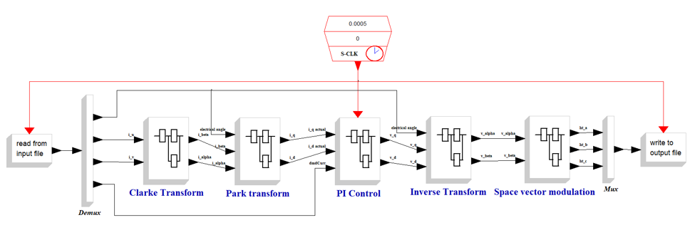
Each block has its own model, such as shown below for the PI Control block.

This PI Control block has two channels for the d and q, each using a common P+I block as shown below.

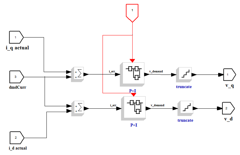
This PI Control block has two channels for the d and q, each using a common P+I block as shown below.

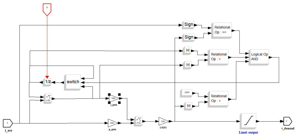
The PI algorithm itself is the bottom left part of this model, the 1/z block being a one cycle delay to add the value of the integral term from the previous execution cycle (the z being the z transform, as this is a discrete (sampled) system).  The remaining part of the model is to prevent integrator “wind-up” and limit the demanded output.

I have modeled using the Scicos graphical notation only. However, modeling tools such as this will also allow blocks that are defined by mathematical expressions, which can be easier in cases where the relationship between input and output can be easily expressed as mathematical equations. 

Note the use of the “truncate” block in these models.  This is introduced because the code is a fixed-point implementation.  We therefore have to quantize the output from our model.

The test harness

I chose to use Google Test because I was curious to try it out. At the current time I haven’t fully developed this test harness. It remains at this time very basic. and requires the input values and expected results to be hard-coded into the test program.

Conclusions

Even when using an open source modeling tool, it proved to be fairly simple to create a model that can be used to generate expected outputs from a control loop. However, that may be because I have had some previous background with using similar techniques. Someone coming to this from a pure programming background may need to spend some time learning to describe algorithms in the form of a model rather than source code.

Modeling the expected output of a fixed-point implementation is more difficult than a floating-point implementation. I took some additional time to introduce quantization into the model to generate the exact same values as the code. It may have been sufficient to just put a range on the test output checking to allow for the fact that the code may generate a slightly different value to the model.

Creating a test harness using Google Test that allows multiple calls to the function being tested proved to be not very straightforward. Although it is possible to put a loop in the test program to make the multiple calls, and to check the outputs, Google Mock calculates the values to be checked only once, so I had to hard-code the expected results in the mock macros, rather than being able to read the expected results from an array as I had hoped. I will continue to dig into this to see if I can find a way.